Welcome in SHADE
Brief overview
SHADE is a Shiny application for providing support to researchers in design of experiments. It includes a tool to perform power analysis for usual test statistics, as well as a reporter tool to draft the ethics committee form for animal experimentation (CETEA), in a user-friendly interface. Initially created to design experiments using animals, SHADE might be used to design any experiments (cell culture…).
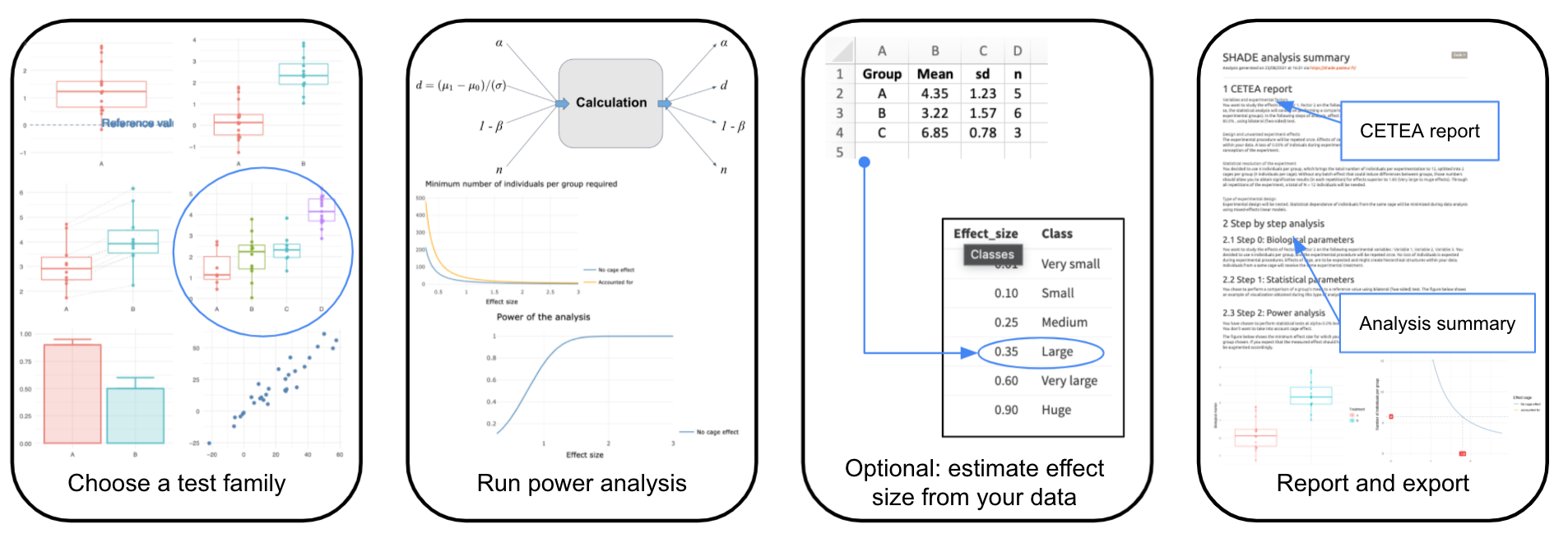
The global workflow of SHADE is detailed hereafter:
What's new in SHADE
Future version is being developped to improve user interface and facilitate navigation
October 2023 - New version of SHADE is online !
User interface improved with an advanced tab for exploring parameters and language option in final report. Cage effect visualisation was also improved.
February 2021 - Version 2.0 released
User interface was improved with validation buttons, tabs for exploring parameters. Bugs were fixed such as external data loading and numerical errors in power analysis.
March 2019 - SHADE is online
Implementing power analysis for frequently used statistical tests, power graph and a report for CETEA form.
Authors
Maintainers and contributors


Acknowledgements


Aim:
SHADE is an application to help scientists refine their experiment design, notably when the design is nested (e.g., animals are collectively bred in cages, etc.). The application proceeds step by step :
- choosing the type of statistical test you want to make (e.g. paired t-test) ;
- exploring and setting parameters of the analysis (preliminary data may be used to estimate effect sizes - see the “optional” sub-step) such as power or sample size;
- making a report. Note that some advanced options are available in a separate page.
Depending on the amount of information you have in hand, you might want to use the application in different manners :
Basic approach : no information available
Partially informed approach : some information is available i.e. standard deviation for at least one experimental group
Refined approach : you have quantities needed to estimate effect size i.e. means and standard deviations for at least 2 experimental groups
How:
Basic approach
–> Level of information : very poor (no preliminary data)
It is not rare for a scientist to start from scratch ! Imagine you have some work contraints (budget, amount of time, room, etc.) and you do not have a guess about the strength of the experimental effect you are studying. In this case, we advise you to estimate the strength of the exprimental effect you will be able to show, given a fixed number of animals. For instance, to study the effects of a factor of interest (group A vs. group B), suppose that you could not use more than \(N\) mice per experimental group (and \(M\) mice per cage) given some work constraints. In this case, the best option is to crudely assess the resolution of your expreriment by estimating the effect size, that is, the minimal size of the experimental effect you may be able to show, given a number of observations per group.
Input parameters involved :
- alpha - controlling the probability of making a mistake by concluding the experimental effect is significant while it is not the case. Also known as Type I Error or False Discovery Rate. It is common to set this parameter at alpha = 0.05.
- beta - controlling the probability to miss a genuine effect by performing a statistical test. If you are not very familiar with this parameter we advise to fix it at beta = 0.8 (i.e., 80% chance you would not miss a genuine experimental effect by performing a statistical test).
- n - the number of individuals per group. Given your own constraints you may have a guess about the number of observations you can reasonably handle.
- if your experimental design is nested (observations are nested within experimental units, e.g., cages, aquariums, petri dishes, etc.), you can make it explicit by ticking the corresponding box and gauge the impact of technical effects. Quantifying these technical effects might be necessary to correctly design your experiment ; they may affect the sample size when their impact is rather substantial.
Output parameter :
- the effect size - a standardized estimate of the strength of the experimental factor under study. See the glossary for the formulas used in SHADE.
Partially informed approach
–> Level of information you have in hand : medium (standard deviation in at least one experimental group)
WIP - Coming soon
Refined approach
–> Level of information : good (means and standard deviations in every experimental groups)
In other contexts, some bits of information may be available. For example, you may be able to guess the strength of the experimental effect you are interested in, (i) based on preliminary data (mean and standard deviation) you have in hand or (ii) simply based on similar experiments that were published on similar study systems. The key estimate here is an “effect size” that reflects the amount of signal in your data (the amount of variation among experimental group) with respect to the amount of noise (technical and/or biological variation within experimental group). In this case, the point will be to (i) estimate the adequate effect size index and then to (ii) calculate a number of individuals based on this effect size index, a desired power (resolution - usually > 80%), and a chosen risk to get a false positive outcome (it is common to set alpha = 0.05). Indeed, depending on the analysis chosen, e.g. “comparing two groups” or “comparing k (k > 2) experimental groups” the effect size will not be estimated using the same metric. See the glossary hereafter for the formulas used in SHADE.
Input parameters involved :
- alpha - controlling the probability of making a mistake by concluding the experimental effect is significant while it is not the case. It is common to set this parameter at alpha = 0.05.
- beta - controlling the probability to miss a genuine effect by performing a statistical test. If you are not very familiar with this parameter we advise to fix it at beta = 0.8 (i.e., 80% chance you would not miss a genuine experimental effect by performing a statistical test).
- the effect size - a standardized estimate of the strength of the experimental factor under study. Based on preliminary data, this parameter value may be estimated with SHADE (see the section “Optional: estimate effect size”).
- if your experimental design is nested (observations are nested within experimental units, e.g., cages, aquariums, petri dishes, etc.), you can make it explicit by ticking the corresponding box and gauge the impact of technical effects. Quantifying these technical effects might be necessary to correctly design your experiment ; they may affect the sample size when their impact is rather substantial.
Output parameter :
- n - the number of individuals per group. By considering technical effects explicitely, you may see the impact of the latter on the initial estimate (i.e., if there were no experimental effect).
Would you need help or guidance regarding an experiment plan, do not hesitate to contact us.
Aim:
The mathematical functions to compute power analysis are specific to each test statistic. Therefore, once clicking on Step1: set test family tab, you may have to chose the type of test statistic you will perform on your data.
How:

(1a) Six statistical tests are available in SHADE. The choice by default is the comparison of two-means for unpaired data (e.g. comparing the body weight of treated and control animals).
(1b) If you chose the comparison of more than two means (Analysis of Variance), you may specify the number of groups to compare. Default is 3 (e.g. 3 doses or 3 timepoints)
(2) Note that a graphical representation of synthetic data appears on the right panel for each test to help for decision. There is a match between data representation and the test statistic associated to it.
(3) Next, you may specify the way to compute statistical significance of your test, aka the type of alternative hypothesis of your test.
By default, a power analysis for a two-sided (or two-tailed) test is performed. Indeed, this option is appropriate if you have no prior knowledge on the direction of the change.
A one-sided (or one-tailed) test is appropriate if the biomarker may depart from the reference (control) value in only one direction, left or right, but not both. An example can be whether animals are fed by a high-fat diet and you expect that the body weight can only increase compared to the control diet, otherwise the diet has no effect. Note that one-sided tests are more powerful.
(4) At the end, a summary of your choices is printed out and you may validate your choices or restore to default settings (comparison of two-means, unpaired, two-sided) before going to the next step Step2: run power analysis.
Note:
- buttons contain more information about the analysis options, do not hesitate to consult them.
Aim:
The second step is there to help you define the parameters for the power analysis in itself. Three main parameters are to be defined in order to estimate the necessary number of individuals per group:
- Type I error
- Power
- Expected experimental effect (magnitude)
Additionally, you can choose to take into account the hierarchical structure of your data by including a cage effect. You'll then have to define the magnitude of this effect and the number of individuals in each cage. Three tabs are available to guide you in the process, and to help you visualize the link between all parameters. If you are unsure of values you want to use, start by exploring the parameters in the second tab. Once you are confident with the values, go back to the first tab to confirm your choices.
How:
- Validate parameters :

In the first box (1a), you have three sliders corresponding to the three parameters you have to define. Default values are given but not necessarily adapted to your analysis.
By clicking on the Account for cage effect checkbox, two more sliders appear to define the magnitude of cage effect and the number of individuals per cage.
Once you have set the values according to your needs, the second box (1b) displays a small summary for you to check.
You can confirm your choices and go to the next step, or restore default values.
- Explore parameters :

This tab is here to help you visualize the meaning of the different parameters you need to define in the first tab.
A first box (2a) allows you to select two variables that will be plotted in the interactive power graph plot (2b).
The four variables of a power analysis are available: type I error (alpha), power, effect size and number of individuals per group.
With the curve, you can for example see which minimum number of individuals is required to obtain a certain level of power.
Two curves will be displayed if you chose to take into account for cage effect : the estimations are impacted by the magnitude of the effect of hierarchical structure.
The second graph (2d) is a simulation adapted to the choices made in Step 1 - set test family.
This graph reacts to the values you set in the box next to it (2c), which contains the same sliders than the validation step, and also impact the power graph interactive plot.
Feel free to move the sliders and see how they modify in the simulation and the power graph. You can also re-run the simulation with the New simulation button.
- Statistical analysis (To go further) :

This last tab is similar to the previous one: it contains once again the same parameters box with the sliders (3a) and a simulated data representation (3b).
On the graph were added the results of a basic statistical test, adapted to the type of analysis you have chosen. The name of the test used and the p-value are reported on the graph.
Like the second tab, this one allows you to explore the impact of each parameters on the simulated data, but this time also showing you their impact on a p-value you would obtain with a typical parametric test.
Additionally, the last box (3c) contains an explanation on hierarchical structure of data, and illustrates the importance of taking those structures into account when performing a statistical analysis.
Aim:
This optional step is there to help you estimate the effect-size in your experiment. If you have no idea about the expected effect-size you can use previous relevant experiments to estimate it.
How:

In SHADE application, there are two ways to estimate the effect size from previous experiments. In the box (1) you can load a xls or xlsx file containing:
Raw data - a two columns file with the results of the experiment (measurements,…) and the groups studied (KO/WT, Drug/No drug …)
Summary statistics - a four colums file with the groups studied, their mean, standard deviation and size.
In (2a) you have an overview of the data format you must load (be careful of the columns orders). Once you have loaded your file, the first few lines appears (2b). If the format does not match SHADE requirements, an error appears in the first box, otherwise the data is loaded successfully. Then click the Estimate effect size button. Shade provides you the estimate effect size, the minimum number of individuals to detect such effect for a given power and significance level (set in Step 2 - run power analysis ) in box (3)

Note:
- You must use similar experiments in terms of groups to be compared, measurements, units…
- The number of groups provided must correspond to the number of groups selected in Step 1 - set test family
A word about effect size:
This panel contains as well a tab What is effect size that explains how the so-called effect size in computed in SHADE. Note that this definition varies according to the test family. Take time to deep your knowledge about it !

Aim:
The last step of the analysis is designed to help you to fill the “statistical and reducing approach” paragraph of the CETEA report (i.e. paragraph 3.3.6.2.Réduction). Of course, this report is general enough to be used in any form where sample size of an experiment must be justified.
How:

(1) The right panel contains a draft of paragraph with four statistical elements that should be described when designing an experiment. On the left panel, you can customize the elements specific to your experiment (primary variables, experimental groups, sample size…). The text on the right is updated accordingly.
(2) If you provided a file into the Optional: estimate effect size tab, the paragraph is enriched with the effect size computed from the loaded data and the sample size needed to achieve this effect size. Nevertheless, you may decide to set in this report a sample size different from the one computed from the loaded data, which will change the associated value of effect size (increasing the sample size decreases the effect size). Then, the paragraph will contain both sample sizes and effect sizes.
(3) By default the report is written in English but you can translate the report in French by clicking on the French flag at the bottom right.
(4) To export the report, you can copy-paste the text directly from SHADE, or download a detailed report by clicking on the “export to HTML” or “export to PDF” buttons. These reports contain all the elements used for the SHADE analysis, the generated graphs and the CETEA report as well.
We gathered here a list of concepts that can be useful to be roughly defined to run a peaceful power analysis.
Effect size
WIP - Coming soon
Cage effect
WIP - Coming soon
How to design an experiment with repetitions?
WIP - Coming soon
Define parameters
First, choose a test family
Save for next steps and send to report
Visual example
Run power analysis
Estimate effect-size with relevant previous experiment
Overview of data format
What is effect size ?
Below is a toy example to illustrate effect size for comparing two proportions, using Type one error α=5% and a power of 80% :
What is effect size ?
Below is a toy example to illustrate effect size for comparing two continuous variables, using Type one error α=5% and a power of 80% :
What is effect size ?
Effect size can be interpreted as the number of standard deviation between the means of the two groups.
Below is a toy example to illustrate effect size for a paired comparison, using Type one error α=5% and a power of 80% :
Make a CETEA report (DAP form) and export it
Specify features of your experiment
ANALYSIS SUMMARY
To contact us
SHADE is an application developed by members of the Hub of Bioinformatics and Biostatistics of the Institut Pasteur.
It provides support to Pasteur research units in Bioinformatics and Biostatistics. The list of the services offered by the Hub are detailed hereafter:
- Short questions : if you have a simple question about bioinformatics and / or statistics, you can ask your question on this website . A mail is sent to all Hub members and one of them will answer you within a few hours.
- Open desk : come and discuss about your data, your project, your analyses or just about bioinformatics and (bio-)statistics every Tuesday morning from 10 to 12 in Yersin Building (24) 1st Floor. Hub members with complementary fields of expertise will be ready to answer your questions and discuss with you.
- Collaborative projects : you are starting a project or you are planning experiments? You need advice and / or help in bioinformatics and (bio-)statistics to design your experiment and analyze your data, or develop a specific software? Please submit a project here . Dedicated Hub members can be involved in your project from the beginning.
You may find more information about the Hub of Bioinformatics and Biostatistics on the team webpage .